Contents

% Tarea de matlab
% Javier Herrero Barrio

Ejercicio 2

A=[4 -2 -10; 2 10 -12; -4 -6 16];
B=[-10; 32; -16];
X=A\B

X =

    2.0000
    4.0000
    1.0000

Ejercicio 4

A=[0 1 -1; -6 -11 6; -6 -11 5];
[X,D]=eig(A)
T1=A*X
T2=X*D

X =

    0.7071   -0.2182   -0.0921
    0.0000   -0.4364   -0.5523
    0.7071   -0.8729   -0.8285


D =

   -1.0000         0         0
         0   -2.0000         0
         0         0   -3.0000


T1 =

   -0.7071    0.4364    0.2762
   -0.0000    0.8729    1.6570
   -0.7071    1.7457    2.4856


T2 =

   -0.7071    0.4364    0.2762
   -0.0000    0.8729    1.6570
   -0.7071    1.7457    2.4856

Ejercicio 5

Y=[1.5-2j -0.35+1.2j; -0.35+1.2j 0.9-1.6j];
I=[30+40j;20+15j];
disp('Solucion: ')
V=Y\I
S=V.*conj(I)

Solucion: 

V =

   3.5902 +35.0928i
   6.0155 +36.2212i


S =

   1.0e+03 *

   1.5114 + 0.9092i
   0.6636 + 0.6342i

Ejercicio 6

hanoi(5,'a','b','c')

mover disco 1 de a a c
mover disco 2 de a a b
mover disco 1 de c a b
mover disco 3 de a a c
mover disco 1 de b a a
mover disco 2 de b a c
mover disco 1 de a a c
mover disco 4 de a a b
mover disco 1 de c a b
mover disco 2 de c a a
mover disco 1 de b a a
mover disco 3 de c a b
mover disco 1 de a a c
mover disco 2 de a a b
mover disco 1 de c a b
mover disco 5 de a a c
mover disco 1 de b a a
mover disco 2 de b a c
mover disco 1 de a a c
mover disco 3 de b a a
mover disco 1 de c a b
mover disco 2 de c a a
mover disco 1 de b a a
mover disco 4 de b a c
mover disco 1 de a a c
mover disco 2 de a a b
mover disco 1 de c a b
mover disco 3 de a a c
mover disco 1 de b a a
mover disco 2 de b a c
mover disco 1 de a a c

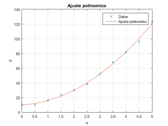
Ejercicio 7

x= 0:0.5:5;
y=[10 10 16 24 30 38 52 68 82 96 123];
p=polyfit(x,y,2)
yc=polyval(p,x);
figure(1)
plot(x,y,'x',x,yc);
xlabel('x'),ylabel('y'),grid,title('Ajuste polinomico')
legend('Datos','Ajuste polinomico',4)

p =

    4.0233    2.0107    9.6783

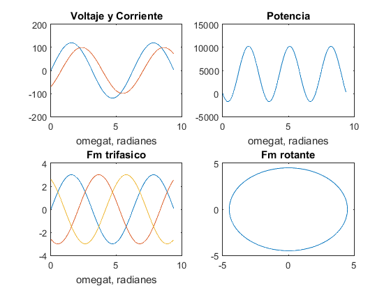
Ejercicio 8

figure(2)
wt=0:0.05:3*pi;
v=120*sin(wt);
i=100*sin(wt-pi/4);
p=v.*i;
subplot(2,2,1)
plot(wt,v,wt,i)
title('Voltaje y Corriente'),xlabel('omegat, radianes')
subplot(2,2,2)
plot(wt,p)
title('Potencia'),xlabel('omegat, radianes')
Fm=3.0;
fa=Fm*sin(wt);
fb=Fm*sin(wt-2*pi/3);
fc=Fm*sin(wt-4*pi/3);
subplot(2,2,3)
plot(wt,fa,wt,fb,wt,fc)
title('Fm trifasico'),xlabel('omegat, radianes')
fR=3/2*Fm;
subplot(2,2,4)
plot(-fR*cos(wt),fR*sin(wt))
title('Fm rotante')

Ejercicio 11

p=[ 1 0 -35 50 24];
r=roots(p)

r =

   -6.4910
    4.8706
    2.0000
   -0.3796

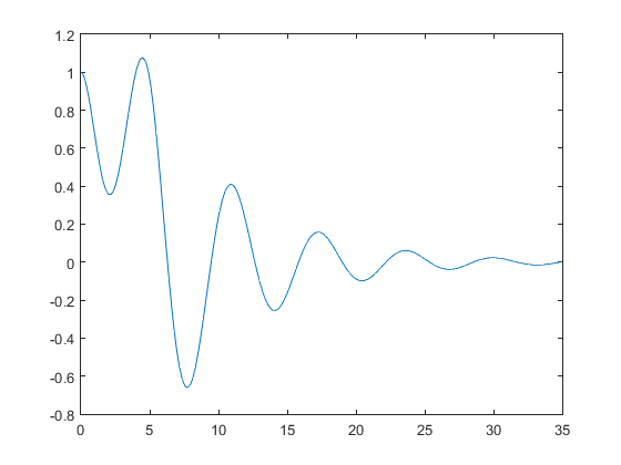
Ejercicio 12

figure(3)
Ejemploode

Ejercicio 13

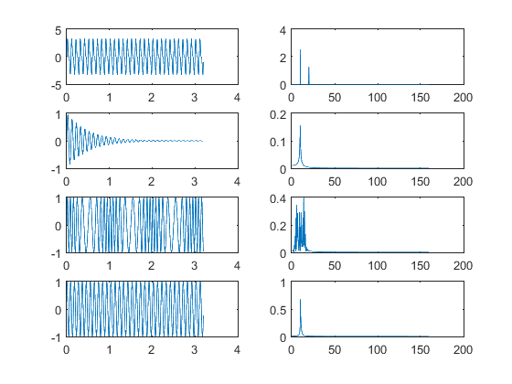
figure(4)
k = 5;   m = 10;   fo = 10;   Bo = 2.5;
N = 2^m;   T = 2^k/fo;
ts = (0:N-1)*T/N;
df = (0:N/2-1)/T;
SampledSignal = Bo*sin(2*pi*fo*ts)+Bo/2*sin(2*pi*fo*2*ts);
An = abs(fft(SampledSignal, N))/N;
subplot(4,2,1)
plot(ts, SampledSignal)
subplot(4,2,2)
plot(df, 2*An(1:N/2))

SampledSignal1 = exp(-2*ts).*sin(2*pi*fo*ts);
An1 = abs(fft(SampledSignal1, N))/N;
subplot(4,2,3)
plot(ts, SampledSignal1)
subplot(4,2,4)
plot(df, 2*An1(1:N/2))

SampledSignal2 = sin(2*pi*fo*ts + 5*sin(2*pi*fo/10*ts));
An2 = abs(fft(SampledSignal2, N))/N;
subplot(4,2,5)
plot(ts, SampledSignal2)
subplot(4,2,6)
plot(df, 2*An2(1:N/2))

SampledSignal3 = sin(2*pi*fo*ts - 5*exp(-2*ts));
An3 = abs(fft(SampledSignal3, N))/N;
subplot(4,2,7)
plot(ts, SampledSignal3)
subplot(4,2,8)
plot(df, 2*An3(1:N/2))

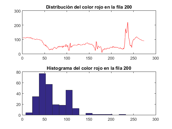
Ejercicio 14

figure(5)
A = imread('WindTunnel.jpg', 'jpeg');
%image(A)
%figure
% row=input('qué fila? ');
row = 200;
red = A(row, :, 1);
gr  = A(row, :, 2);
bl  = A(row, :, 3);
subplot(2,1,1)
plot(red, 'r');
title('Distribución del color rojo en la fila 200');
%hold on
%plot(gr, 'g');
%plot(bl, 'b');
subplot(2,1,2)
hist(red,0:15:255);
title('Histograma del color rojo en la fila 200');

Published with MATLAB® R2015a